In the context of multivariable linear regression, leverage is a distance measure that shows how far an observation is from the center of the multivariate predictor space. Observations with high leverage values would have the potential to influence the regression model highly while observations with low leverage values would not. Additionally, leverage can be used to determine if a new observation is close to the predictor space of the observations used to create the model in order to avoid extrapolation.
Once a linear regression model is built, we can get the leverage values of all the observations used in the model from the diagonal values of its hat matrix. However, a key point to remember is that leverage as a measure of distance is not Euclidean, so we shouldn’t expect the distance to be a straight line to the center of the multivariate predictor space. Instead, leverage takes into consideration the predictor correlations and is therefore able to detect multivariate outliers — which are outliers in the full predictor space taken together though they may not be outliers for any predictors individually!
The following example demonstrates the idea. Let’s say we have 17 labeled observations in the predictor space consisting of 2 predictors \(x_1\) and \(x_2\). The below scatter plot shows the predictor space:
library(tidyverse)
theme_set(theme_bw())

df <-tibble(x1=c(1,2,3,4,5,6,7,8,9,10,11,12,13,14,15,11,25),
            x2=c(2,2.5,3.2,4.6,5.3,6.4,7.9,8.4,9.3,10.2,11.5,12.3,13.7,14.1,15.6,4,26),
            y=c(1,3,2,4.3,5.3,7.3,6.1,8.8,9.3,10.9,11.1,12.5,13.2,14.9,15.8,5,25.4),
            obs=1:17)

ggplot(df, aes(x1, x2)) + geom_point() +
  geom_label(aes(label = obs), nudge_y = 2) +
  scale_x_continuous(breaks = seq(0, 25, 5)) +
  scale_y_continuous(breaks = seq(0, 25, 5)) +
  labs(title = "Our Predictor Space", x = expression("x"[1]), y = expression("x"[2]))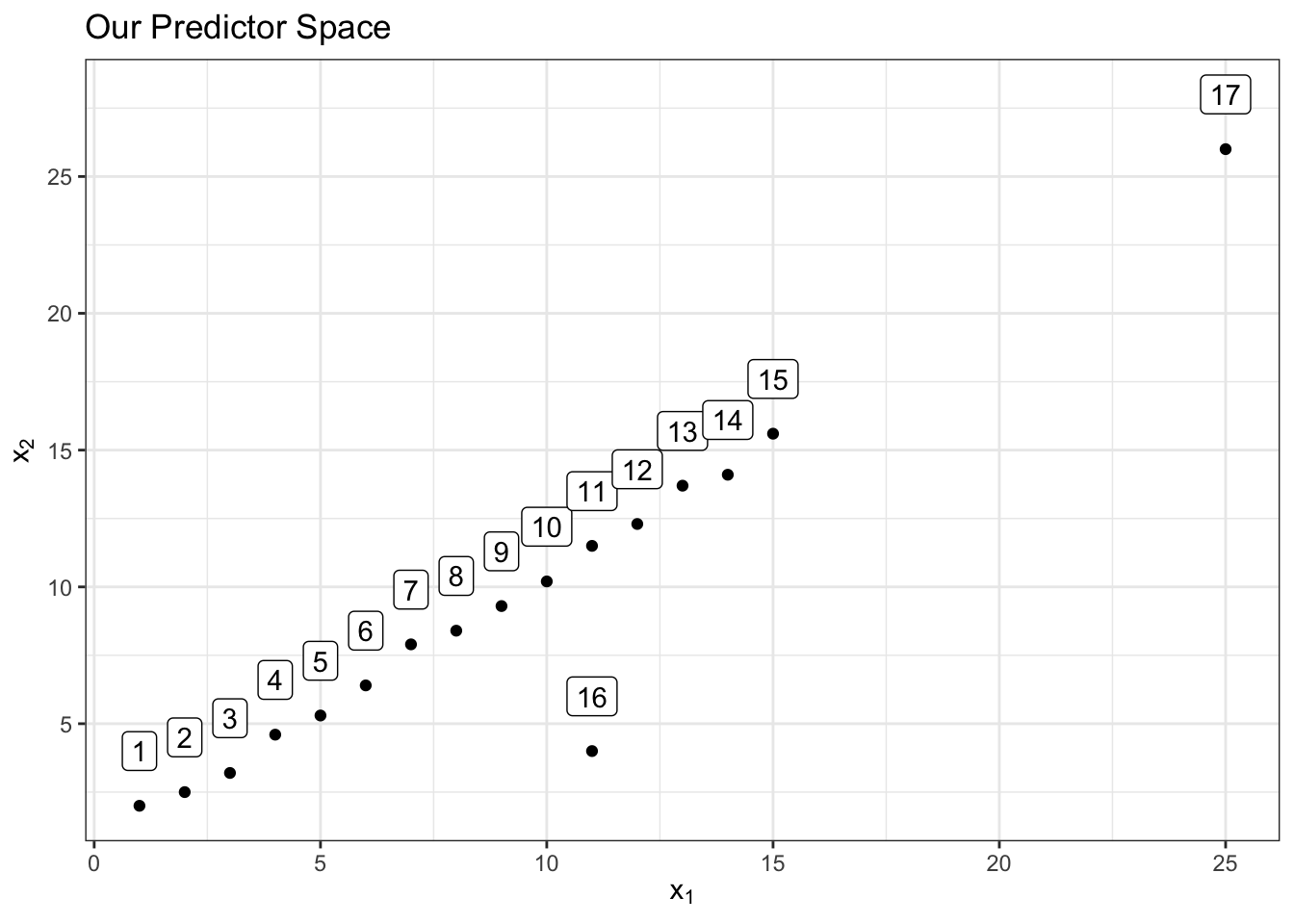
Notice that observation 16 above is not an outlier in the \(x_1\) space by itself or in the \(x_2\) space by itself. However, it is a multivariate outlier in the predictor space of \(x_1\) and \(x_2\) together since it’s out of the “oval” region that those 2 predictors have together which is represented below with an 80% confidence level ellipse for demonstrative purposes:
ggplot(df, aes(x1, x2)) + geom_point() +
  geom_label(aes(label = obs), nudge_y = 3) +
  scale_x_continuous(breaks = seq(0, 25, 5)) +
  scale_y_continuous(breaks = seq(0, 30, 5)) +
  stat_ellipse(level = 0.80) +
  labs(title = "Our Predictor Space", x = expression("x"[1]), y = expression("x"[2]))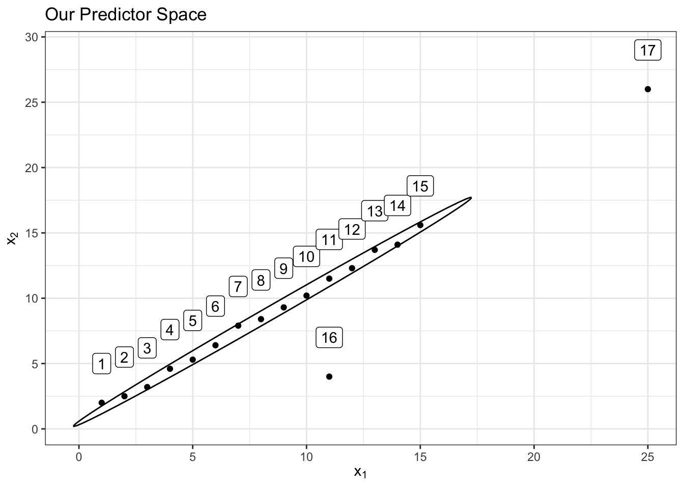
Observation 17 above on the other hand is an outlier in both the \(x_1\) and \(x_2\) predictor spaces separately and also an outlier to the region of both predictors together since it’s far away from the center of the multivariate predictor space despite being true to the correlation relationship between the predictors.
Now let’s fit a linear model between a third variable \(y\) as the outcome and our variables \(x_1\) and \(x_2\) as predictors. The model equation will therefore be: \[\hat{y} = b_0 + b_1x_1 + b_2x_2\]
Below is a bar plot showing the leverage of the observations in the model:
model <- lm(y ~ x1 + x2, data = df)

lev_obs <- tibble(leverage = hatvalues(model), obs = 1:17)

ggplot(lev_obs, aes(obs, leverage)) + geom_col() +
  scale_x_continuous(breaks = seq(1, 17)) +
  labs(title = "Observation Leverage Values", x = "Observation", y = "Leverage")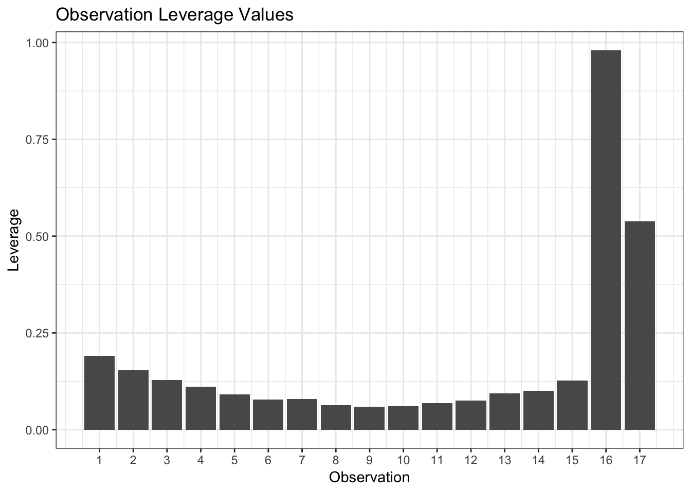
Notice how the leverage metric (from the diagonal of the hat matrix) was able to successfully detect that both observations 16 and 17 were far from center of the multivariate oval region of the predictors.
Observations that are not outliers for the predictors individually but are outliers for the predictors when taken together (the oval) will still be detected by the leverage metric. Therefore, when we have a new observation that we want to predict (\(h_0\)), we need to make sure that its leverage is less than the maximum leverage value (\(h_{max}\)) used in the model to ensure it’s within the multivariate predictor region covered by the model and that no extrapolation will take place.
Tangentially, the Mahalanobis distance is a similar distance measure that we can use for the same purpose as it can also measure distances from the center of multivariate predictor regions where predictor correlations are also taken into account. It is also very easy to calculate for new observations and compare to the Mahalanobis distances of the observations used in a model.
Below are the Mahalanobis distances of our example above:
df_temp <- select(df, x1, x2)

means <- colMeans(df_temp)
cov_matrix <- cov(df_temp)

mahalanbis_distances <- mahalanobis(df_temp, means, cov_matrix)

mh <- tibble(obs = 1:17, maha = mahalanbis_distances)

ggplot(mh, aes(obs, maha)) + geom_col() +
  scale_x_continuous(breaks = seq(1, 17)) +
  labs(title = "Observation Mahalanobis Distance Values",
       x = "Observation", y = "Mahalanobis Distance")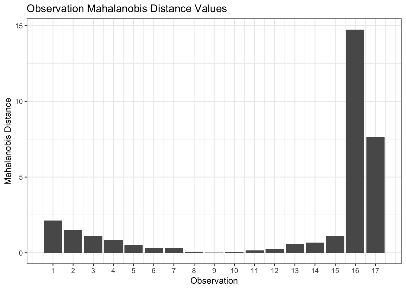
Notice that while the Mahalanobis distance values are different from the leverage values, the shape of the plot is identical which indicates that we are measuring the same phenomenon. Therefore, we should be able to compare either metric for a new observation to the maximum value of that metric in our data to determine if we are extrapolating or not. However, this can be misleading if our model is not free from outliers such as in our example above. In such cases, we may better assess it by determining how many multiples of the average metric value (leverage or Mahalanobis distance) this new observation is. If observations 16 and 17 had been excluded before building the model, then comparing it to the maximum metric value would be sensible.
In fact, leverage and the Mahalanobis distance are related through the equation: \[ \text{Mahalanobis}_i=(N-1)(H_{ii}-\frac{1}{N})\]
where:
- \(N\) is the total number of observations used in the model
- \(H_{ii}\) is the diagonal value of the hat matrix of the model providing the leverage value of observation \(i\)