Businesses face various types of problems that require making optimal decisions in order to achieve a certain objective. One such problem is the transportation / assignment problem I came across when I was reading the excellent “Spreadsheet Modeling and Decision Analysis” book by Cliff T. Ragsdale. I found this type of problem interesting because the concept can be generalized to many areas of the business.
In this post, I will discuss a transportation / assignment problem scenario where we need to select the optimal supply sources & routes that would meet as much of the demand as possible while minimizing the cost of shipping. I will use network modeling & linear programming with Gurobi Python to model & solve this problem.
An electronics company has decided to build 3 factories for its flagship product. There are 4 cities being considered as locations for those factories — Boston, Miami, Seattle, and Los Angeles. A maximum of one factory can be built in a city and each factory option has a different production capacity.
Additionally, the company has identified 4 cities with high demand for its products — Minneapolis, Chicago, Denver, and Dallas. The shipping cost per unit differs depending on the origin & destination cities.
The production capacities, demand levels, & shipping costs are in the table below:
| Demand Cities | Boston | Miami | Seattle | Los Angeles | Demand |
|---|---|---|---|---|---|
| Minneapolis | $20 | $24 | $22 | $26 | 4500 |
| Chicago | $18 | $20 | $23 | $24 | 7000 |
| Denver | $24 | $25 | $16 | $15 | 4500 |
| Dallas | $23 | $17 | $23 | $17 | 5500 |
| Supply | 3500 | 5000 | 4000 | 6000 |
Notice that the total demand of the demand cities exceeds the total supply of all 4 potential factories of which we can only select 3.
We need to decide which 3 cities should be selected for the factories as well as which routes should be used from each of them (& the number of units to ship) in order to minimize the cost of shipping while meeting as much of the demand as possible.
The information in the above table can be visualized as a network plot. We’ll use visNetwork, which is a great R package for interactive network visualization.
The production capacity values of the supply nodes are represented by negative values while the demand values of the demand cities are represented by positive values.
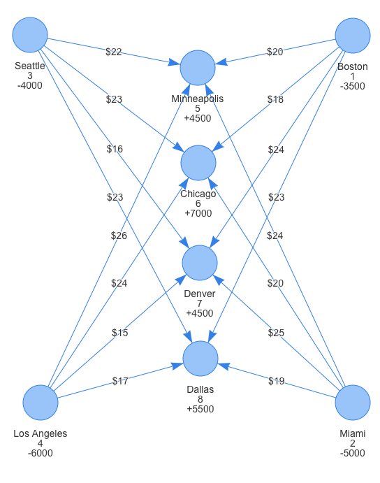
Note that we’re not just trying to distribute our supply at the cheapest cost possible but rather trying to meet as much of the demand as possible with the least shipping costs.
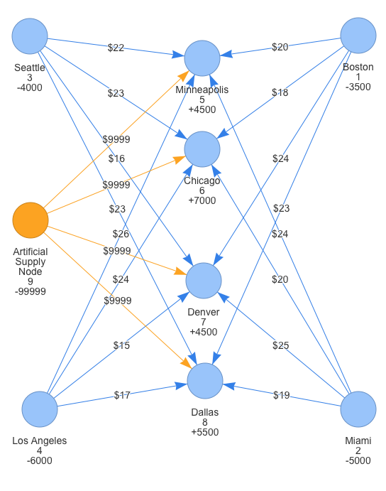
If we try to solve this problem directly and minimize shipping costs, the model might prefer factories with smaller production capacities since distributing their supply may result in lower shipping costs. However, that would meet less of the demand, and our objective will not be achieved. To meet as much of the demand as possible at the lowest possible cost, we need to introduce an artificial supply node with an arbitrarily large supply quantity and large shipping cost per unit for all its possible routes. This addition makes our total supply exceed the total demand and would therefore force the model to fill as much of the demand as possible and would use the supply from the artificial node when it absolutely needs it (since it has very high costs). We can then ignore the parts of the solution related to the artificial supply node and its routes but use the remaining parts of the solution.
The new network model is shown below:
Mathematical Formulation & Model Building
Let’s formulate the model mathematically and build the model with Gurobi Python.
Decision Variables
There are two groups of decision variables needed here. First, a group of binary decision variables, one for each of the supply cities that would take a value of 1 if that city is selected and 0 otherwise. Second, a group of integer decision variables that represent the number of units to send for each possible route. If that value is 0, then the route will not be used. These can be represented mathematically as:
Binary variables that equal 1 if if node \(i\) is selected as a supply node:
\(y_i ~\forall ~i \in \{1,2,3,4\}\)
The number of units to send from supply node \(i\) to demand node \(j\):
\(x_{ij} ~\forall ~i \in \{1,2,3,4,9\}, ~j \in \{5,6,7,8\}\):
Let’s create those decision variables in our Gurobi Python model:
from gurobi import *

m = Model("M1") # Setting up the model

# Creating the decision variables

y1 = m.addVar(name = "y1", vtype=GRB.BINARY) # Will node 1 be used for supply? 1/0
y2 = m.addVar(name = "y2", vtype=GRB.BINARY) # Will node 2 be used for supply? 1/0
y3 = m.addVar(name = "y3", vtype=GRB.BINARY) # Will node 3 be used for supply? 1/0
y4 = m.addVar(name = "y4", vtype=GRB.BINARY) # Will node 4 be used for supply? 1/0
x15 = m.addVar(name = "x15", vtype=GRB.INTEGER) # Num. units sent from node 1 to node 5
x16 = m.addVar(name = "x16", vtype=GRB.INTEGER) # Num. units sent from node 1 to node 6
x17 = m.addVar(name = "x17", vtype=GRB.INTEGER) # Num. units sent from node 1 to node 7
x18 = m.addVar(name = "x18", vtype=GRB.INTEGER) # Num. units sent from node 1 to node 8
x25 = m.addVar(name = "x25", vtype=GRB.INTEGER) # Num. units sent from node 2 to node 5
x26 = m.addVar(name = "x26", vtype=GRB.INTEGER) # Num. units sent from node 2 to node 6
x27 = m.addVar(name = "x27", vtype=GRB.INTEGER) # Num. units sent from node 2 to node 7
x28 = m.addVar(name = "x28", vtype=GRB.INTEGER) # Num. units sent from node 2 to node 8
x35 = m.addVar(name = "x35", vtype=GRB.INTEGER) # Num. units sent from node 3 to node 5
x36 = m.addVar(name = "x36", vtype=GRB.INTEGER) # Num. units sent from node 3 to node 6
x37 = m.addVar(name = "x37", vtype=GRB.INTEGER) # Num. units sent from node 3 to node 7
x38 = m.addVar(name = "x38", vtype=GRB.INTEGER) # Num. units sent from node 3 to node 8
x45 = m.addVar(name = "x45", vtype=GRB.INTEGER) # Num. units sent from node 4 to node 5
x46 = m.addVar(name = "x46", vtype=GRB.INTEGER) # Num. units sent from node 4 to node 6
x47 = m.addVar(name = "x47", vtype=GRB.INTEGER) # Num. units sent from node 4 to node 7
x48 = m.addVar(name = "x48", vtype=GRB.INTEGER) # Num. units sent from node 4 to node 8
x95 = m.addVar(name = "x95", vtype=GRB.INTEGER) # Num. units sent from node 9 to node 5
x96 = m.addVar(name = "x96", vtype=GRB.INTEGER) # Num. units sent from node 9 to node 6
x97 = m.addVar(name = "x97", vtype=GRB.INTEGER) # Num. units sent from node 9 to node 7
x98 = m.addVar(name = "x98", vtype=GRB.INTEGER) # Num. units sent from node 9 to node 8
m.update() # Updating the model
Objective Function
We need to calculate the product of the cost of shipping per unit for each route by the number of units to be sent on that route and mimize the sum of those values.
Therefore, the objective function can be expressed mathematically as:
Minimize: \(z = 20x_{15} + 18x_{16} + 24x_{17} + 23x_{18} +\)
\(~~~~~~~~~~~~~~~~~~~~~~24x_{25} + 20x_{26} + 25x_{27} + 17x_{28} +\)
\(~~~~~~~~~~~~~~~~~~~~~~22x_{35} + 23x_{36} + 16x_{37} + 23x_{38} +\)
\(~~~~~~~~~~~~~~~~~~~~~~26x_{45} + 24x_{46} + 15x_{47} + 17x_{48} +\)
\(~~~~~~~~~~~~~~~~~~~~~~9999x_{95} + 9999x_{96} + 9999x_{97} + 9999x_{98}\)
Let’s add this objective function to our Gurobi Python model:
# Setting up the objective function
m.setObjective(20*x15 + 18*x16 + 24*x17 + 23*x18 + 24*x25 + 20*x26 + 25*x27 + 17*x28 + 22*x35 + 23*x36 + 16*x37 + 23*x38 + 26*x45 + 24*x46 + 15*x47 + 17*x48 + 9999*x95 + 9999*x96 + 9999*x97 + 9999*x98, GRB.MINIMIZE)

m.update() # Updating the model
Constraints
Balance of Flow Constraints
This constraints group ensures a balance of flow in our network. Since our total supply now exceeds the total demand, we need to place a constraint for each node such that its Inflow - Outflow \(\ge\) its Supply or Demand.
In our case, all the supply nodes have only outflow and all of our demand nodes have only inflow.
\(-x_{15} - x_{16} - x_{17} - x_{18} \ge -3500\) \(~~~~~~~~~~~~\)} Node 1 \(-x_{25} - x_{26} - x_{27} - x_{28} \ge -5000\) \(~~~~~~~~~~~~\)} Node 2 \(-x_{35} - x_{36} - x_{37} - x_{38} \ge -4000\) \(~~~~~~~~~~~~\)} Node 3 \(-x_{45} - x_{46} - x_{47} - x_{48} \ge -6000\) \(~~~~~~~~~~~~\)} Node 4
\(x_{15} + x_{25} + x_{35} + x_{45} + x_{95} \ge 4500\) \(~~~~~~~~\)} Node 5 \(x_{16} + x_{26} + x_{36} + x_{46} + x_{96} \ge 7000\) \(~~~~~~~~\)} Node 6 \(x_{17} + x_{27} + x_{37} + x_{47} + x_{97} \ge 4500\) \(~~~~~~~~\)} Node 7 \(x_{18} + x_{28} + x_{38} + x_{48} + x_{98} \ge 5500\) \(~~~~~~~~\)} Node 8
\(-x_{95} - x_{96} - x_{97} - x_{98} \ge -99999\) \(~~~~~~~~~~\)} Node 9 (Artificial Supply Node)
Selection of Supply Nodes Constraints
Since we need to select 3 supply nodes out of 4, we need constraints on those nodes to ensure that each of their respective binary decision variables gets set to 1 if any of its supplies are sent on any routes to the demand nodes. This is done by using the equation Outflow + Supply*Binary Var \(\le0\) for each supply node.
\(x_{15} + x_{16} + x_{17} + x_{18} -3500y_1 \le 0\) \(~~~~~~~~\)} Node 1 Binary \(x_{25} + x_{26} + x_{27} + x_{28} -5000y_2 \le 0\) \(~~~~~~~~\)} Node 2 Binary \(x_{35} + x_{36} + x_{37} + x_{38} -4000y_3 \le 0\) \(~~~~~~~~\)} Node 3 Binary \(x_{45} + x_{46} + x_{47} + x_{48} -6000y_4 \le 0\) \(~~~~~~~~\)} Node 4 Binary
Looking at the above inequalities, note that since supply is a negative number, this forces the binary variable for a supply node to become 1 if any of that node’s routes is set to carry any units.
Next, to ensure that 3 supply nodes only are selected we need to add the following constraint:
\(y_1 + y_2 + y_3 + y_4 = 3\)
Non-negativity, Integrality, & Binary Constraints
These constraints ensure that the decision variables can only take on values that make sense in our model.
\(y_i \in \{0,1\} ~\forall ~i \in \{1,2,3,4\}\) \(~~~~~~~~~~~~~~~~~~~~~~~~~~~~~~~~\)} Binary Constraints \(x_{ij} \ge 0 ~\forall ~i \in \{1,2,3,4,9\}, ~j \in \{5,6,7,8\}\) \(~~~~~~~~\)} Non-negativity Constraints \(x_{ij} \in \mathbb{Z} ~\forall ~i \in \{1,2,3,4,9\}, ~j \in \{5,6,7,8\}\) \(~~~~~~~~\)} Integrality Constraints
We have already set the non-negativity, integrality, & binary constraints in our model while we were creating the decision variables. Now, we shall add the rest of the constraints to our model:
# Adding the constraints to the model
m.addConstr(-x15 - x16 - x17 - x18>=-3500, "c1") # Constraint for node 1
m.addConstr(-x25 - x26 - x27 - x28>=-5000, "c2") # Constraint for node 2
m.addConstr(-x35 - x36 - x37 - x38>=-4000, "c3") # Constraint for node 3
m.addConstr(-x45 - x46 - x47 - x48>=-6000, "c4") # Constraint for node 4

m.addConstr(x15 + x25 + x35 + x45 + x95>=4500, "c5") # Constraint for node 5
m.addConstr(x16 + x26 + x36 + x46 + x96>=7000, "c6") # Constraint for node 6
m.addConstr(x17 + x27 + x37 + x47 + x97>=4500, "c7") # Constraint for node 7
m.addConstr(x18 + x28 + x38 + x48 + x98>=5500, "c8") # Constraint for node 8

m.addConstr(-x95 - x96 - x97 - x98>=-99999, "c9") # Constraint for node 9

# Setting the binary var. y1 to 1 if either x15, x16, x17, or x18 are >= 0 else it's 0
m.addConstr(x15 + x16 + x17 + x18 -3500*y1<=0, "c10")

# Setting the binary var. y2 to 1 if either x25, x26, x27, or x28 are >= 0 else it's 0
m.addConstr(x25 + x26 + x27 + x28 -5000*y2<=0, "c11")

# Setting the binary var. y3 to 1 if either x35, x36, x37, or x38 are >= 0 else it's 0
m.addConstr(x35 + x36 + x37 + x38 -4000*y3<=0, "c12")

# Setting the binary var. y4 to 1 if either x45, x46, x47, or x48 are >= 0 else it's 0
m.addConstr(x45 + x46 + x47 + x48 -6000*y4<=0, "c13")

# Ensuring that 3 of the variables y1, y2, y3 and y4 are equal to 1
m.addConstr(y1+y2+y3+y4==3, "c14")

m.update() # Updating the model
Results
Finally, let’s run the optimization and find the optimal values of our decision variables:
m.optimize() # Finding the optimal solution## Optimize a model with 14 rows, 24 columns and 64 nonzeros
## Variable types: 0 continuous, 24 integer (4 binary)
## Coefficient statistics:
## Matrix range [1e+00, 6e+03]
## Objective range [2e+01, 1e+04]
## Bounds range [1e+00, 1e+00]
## RHS range [3e+00, 1e+05]
## Found heuristic solution: objective 2.149785e+08
## Presolve removed 5 rows and 0 columns
## Presolve time: 0.15s
## Presolved: 9 rows, 24 columns, 44 nonzeros
## Variable types: 0 continuous, 24 integer (4 binary)
##
## Root relaxation: objective 6.525850e+07, 15 iterations, 0.04 seconds
##
## Nodes | Current Node | Objective Bounds | Work
## Expl Unexpl | Obj Depth IntInf | Incumbent BestBd Gap | It/Node Time
##
## * 0 0 0 6.525850e+07 6.5258e+07 0.00% - 0s
##
## Explored 0 nodes (15 simplex iterations) in 0.36 seconds
## Thread count was 8 (of 8 available processors)
##
## Solution count 2: 6.52585e+07 2.14978e+08
##
## Optimal solution found (tolerance 1.00e-04)
## Best objective 6.525850000000e+07, best bound 6.525850000000e+07, gap 0.0000%m.printAttr("X") # Printing the decision variable values##
## Variable X
## -------------------------
## y2 1
## y3 1
## y4 1
## x26 5000
## x37 4000
## x47 500
## x48 5500
## x95 4500
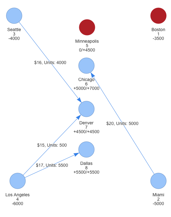
## x96 2000The above solution shows that Miami, Seattle, and Los Angeles (nodes, 2,3,4) have been selected as the 3 supply nodes. We can also see that some routes from those supply nodes were assigned values while others were not. The artificial supply node was also used to fulfill some demand — routes \(x_{95}\) and \(x_{96}\). We should ignore the values related to the artificial node as well as the objective function value in the output since the model only used them to be able to fulfill the demand we could not cover with our real supply. Additionally, the results above show that we could not cover Minneapolis as no routes from Miami, Seattle, or Los Angeles to Minneapolis were assigned positive values. It was simply not economical to fulfill Minneapolis’s demand given that the demand of cities closer to the supply nodes would already exhaust the entire supply of the supply nodes. Chicago’s demand was not even fully met.
The above decision variable values allow us to meet as much of the demand as possible (15000 units) at the lowest cost of shipping: \(20*5000 + 16*4000 + 15*500 + 17*5500=\) $265,000.
The network given by the solution can be seen in the network plot below:
Extensions to the techniques shown here can be used to solve other types of problems including transhipment problems (where some nodes can both send and receive units from other nodes) and shortest path problems (where the objective is to find the shortest path from an origin node to a destination node with multiple nodes and route options between them). Additionally, non-linear programming can be used when the objective functions and/or constraints are non-linear.
Have you come across similar problems in your line of work where using these techniques is needed to reach the optimal solution?
Please share your thoughts in the comments.